As an engineer in the field of computer science, I have recently been heavily studying various machine learning topics at the department of computer science at ETH Zurich. I am convinced that you have to understand this area if you want to stay on top of technology.
After all the theory, it was now about putting what I had learned into practice.
As a small example to start with, I wanted to train a small Convolutional Neural Network (CNN), which is supposed to take a picture and distinguish whether it shows a cat or a dog. In other words: The “hello world” of CNN.
To declare it right from the beginning: I failed miserably.
But I’ve nevertheless learned a lot of stuff.
Setup
- As already mentioned, I approached this task with a CNN.
The framework of my choice is Keras. - The programming language is clear: Python.
- For the training you need a lot of pictures that are labelled. I.e. for all the images it shall be known whether it shows a cat or a dog. Fortunately, there are a lot of data sets available.
The data set of my choice is Dogs vs. Cats from Kaggle. This data set contains about 20’000 pictures of dogs and cats – more than enough for my first steps. - It would be nice to have GPU support, the training is massively faster than without (depending on the task it is more than 100 times faster). Unfortunately, the GPU of my old laptop is not supported.
Network Architecture
I defined the network closely aligned to “Deep Learning with Python“, a book by François Chollet, the creator of Keras.
Because of my old computer without GPU support I had to limit myself to a relatively small network.
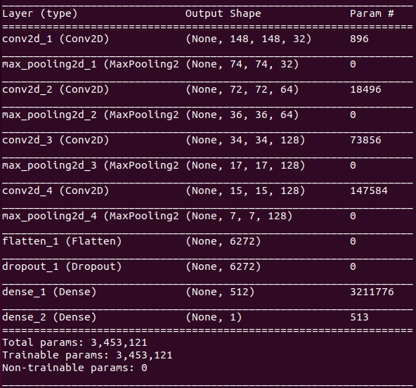
Basically, I just have 4 convolutional 2D layers, each followed by a pooling layer. At the end of the process chain, I flatten and have 2 dense layers. The last layer having just 1 output: In this case the probability that the image shows a dog.
To increase generalization, i.e. to prevent the network from learning all examples by heart, I have also added a dropout layer.
The result is the following CNN with almost 3.5 millions of trainable weights:
Training
The complete data set from Kaggle was way too big for my old laptop. Because with the whole set I would have had to make my network much bigger. Otherwise it would have overfitted for sure.
That’s the reason why I trained my CNN on the basis of a small subset. I had first randomly selected 2’000 images for training and 1’000 more images for validation.
But soon it was clear, that with this sizing I could not get satisfactory results. To mittigate this, I could have just selected more images. But that was too easy. I wanted to get by with just this small set of data.
So I hoped to achieve a higher accuracy by means of data augmentation. That means, I extended the set of images for training with versions of these images, which I rotated, scaled and mirrored.
This is a common procedure to deal with the problem of little data.
Now the actual training could begin. I decided to train the CNN in 100 epochs, each with 100 batches per epoch.
  steps_per_epoch=100
  epochs=100
The whole training lasted almost 20 hours, during which my laptop ran at full throttle on all cores. Afterwards it was time for a first analysis.
Accuracy and Loss
If you have to measure the quality of your CNN, you have to evaluate two things: accuracy and loss. The following figures show how these two KPIs evolved over the 100 epochs of the training.
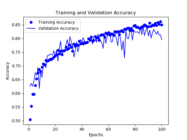
The training accuracy increases over the whole training. However, the validation accuracy is coming to a saturation after 80 epochs. The CNN starts to overfit. I.e. it learns the training images instead of generalized patterns.
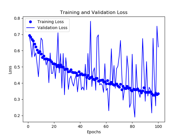
Not surprisingly, also the training loss improves over the whole training. But the validation loss looks a bit like a mess… and remains at a relatively high level.
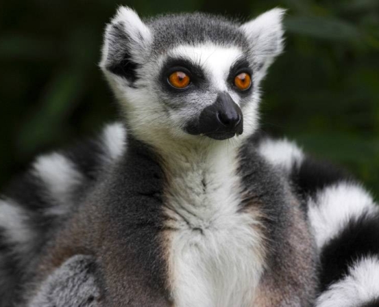
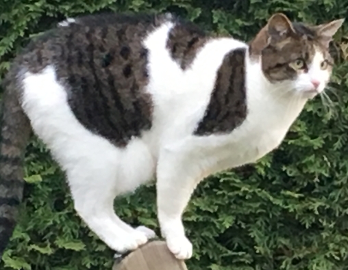
After these findings I was curious to see what this CNN now says about a picture of my cat. I had not used this picture before, neither for training nor for validation. Of course I hoped that the cat would not be categorized as a dog.
Result and Analysis

The picture shows a cat with a probability of 0%
Oh come on!
That is disappointing!
A cat with 0%, therefore a dog with 100% probability!
I wanted to find out where my CNN failed. You sometimes hear that neural networks are black boxes and that the reason for their decision is never clear.
Fortunately, that’s not the case for convolutional networks.
The keyword here is Gradient-Weighted Class Activation Mapping (CAM). This is an algorithm that provides a visual explanation of a deep network. You can calculate a heatmap that highlights the relevant parts of the image. This heatmap you can superimpose with the original image.
I implemented this algorithm and applied it to my CNN.
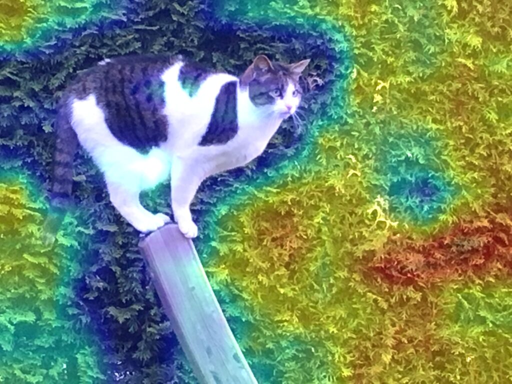
The interpretation is simple: The redder an area is shown in the superimposed picture, the more relevant it was for the network’s decision. The blue areas, however, were irrelevant.
Surprisingly, my CNN ignored the very area with the cat! And it must have interpreted the hedge as the fur of a dog.
In conclusion, this experiment has failed thoroughly!
I showed the same picture to the VGG16 CNN, which was trained using the data in ImageNet. The answer was also not quite correct – although somehow more reasonable: A Madagascar Cat.
Room for Improvement
How can quality be improved?
The two most obvious ways are a) a larger network and b) more data for training. A slightly more elaborate but perhaps more promising approach would be to optimize the architecture.
Finally, what I have done is to manipulate the image. Of course this is not an appropriate approach to improve the quality of the CNN’s prediction, because CNN should be able to handle all images.
But I was interested to see how my CNN reacts to clearer images.
Here come the 3 variants and their recognition rate:
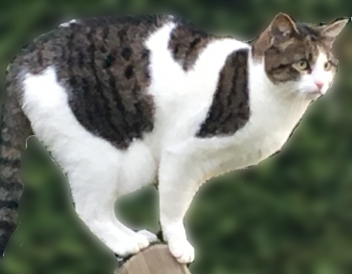
Take the Section with the Cat
The picture shows a cat with a probability of 23%
Cool! It could already be a cat. Let’s take it one step further.
Take the Section with the Cat – and Blur the Background
The picture shows a cat with a probability of 60%
Even better! We slowly get to the point. Let’s take another step.
Take the Section with the Cat – and Remove the Background
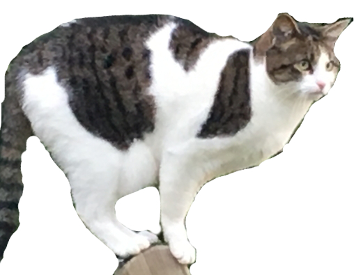
The picture shows a cat with a probability of 84%
Now it’s a cat.